Three musicians are sitting in a bar . . .

. . . in Austria. At 3:00AM. The topic turns to “Funny titles for music”. We aren’t talking about the usual titles like “If You Won’t Leave Me, I’ll Find Somebody Who Will” by Warren Zevon, “Shoop Shoop Diddy Wop Cumma Cumma Wang Dang” by Monte Video and the Casettes, or “Satan Gave Me a Taco” by Beck. We are throwing out titles that could put you into a major existential crisis. Unfortunately, only one stuck with me, “The Negative Space of Speed” that I subtitled “A Musical Null Set“.

Returning from Austria I felt that this title/subtitle needed to actually exist as a piece of music. What I soon realized is there is no possible combination of pitches, rhythms, dynamics, and tempi that could adequately describe this piece. The title implies “not music” or the absence of music. From this realization I managed to score the work for a full wind symphony (minus the piano and harp).

The beauty of the work is its flexibility. It requires NO rehearsal, can be played with ANY combination of wind and percussion instruments, and the musician’s skill level is completely irrelevant. It can also be used to pad an otherwise sparse concert repertoire.

Let’s say that you’ve programmed your concert for six works. But one of the works will have to be cut. There are any number of reasons this could happen:

  • you discovered that you don’t have performance rights to the work
  • the guest soloist turns out to be a serial killer and is arrested the day before the performance
  • the Fire Marshall rules that you can’t play your pyrophone in the concert hall
  • or, the band just can’t play the music.

No problem. Pull the work and replace it with “The Negative Space of Speed“. Your program still has six works and it appears you’re playing a cool Avant-garde 21st century work. Which you are . . . at least conceptually.

Please note that this is not an homage to (or blatant ripoff of) 4’33”, John Cage’s work that explores the idea that segments of time can be filled with structured or ambient sound (noise). Both can be considered music. Additionally, Cage was interested in the behavior of the audience and how their actions contribute to the music.

The Negative Space of Speed” plays with the idea of zero duration. Without duration there can be no music – structured or otherwise. BUT oddly enough, there can still be performance. The conductor turns the page to the score, cues the ensemble, and the audience eagerly anticipates the downbeat of this new piece. What they don’t realize is they missed the piece entirely and the downbeat is for the next work on the list (probably “First Suite in E-flat for Military Band” by Gustav Holst). While this may not cause a near riot as did the premiere of Stravinsky’sThe Rite of Spring” it hopefully will fuel a lively audience discussion of what constitutes music.

And yes, you too can add “The Negative Space of Speed” to your repertoire. The perpetrators of this work have decided to make it a free download!! Just click here.


Electronic Brain Droppings

I’m finally learning the electronics that I should of learned 40 years ago. I did a bunch of Heathkit projects (Heathkit is still around but a shadow of their previous selves.) including my entire stereo system but I never delved too deeply into the theory of how the circuits worked. So now I’m back studying circuit theory, operational amplifiers, first-order filters, and an entire zoo of 21st century electronics design. (That integrated circuit does ALL of that!?!)

Having designed a UV densitometer for my photographic work I’m already thinking about a second, more sophisticated, version. I’m also wanting to explore musical vibrato from the standpoint of what repetition and depth frequencies people find pleasing. Both of these will require some careful design work.

One thing I’ve already had to deal with is non-standard resistor values. When working with operational amplifiers there are sets of equations used to calculate resistor or capacitor values. Since I have a bigger collection of resistors than capacitors it’s easier for me to fix the capacitor value and calculate the resistor value(s) I need. Of course these calculated values are generally no where near the standard resistor values. Figuring out which combination of resistors will get you closest to 27,658 ohms gets very tedious. So being a retired programmer I did what any programmer would do . . . I wrote a python script to find the combinations for me. (View the source code here.)


A note to any programmers who may look at this code.

I don’t care that I’m not using some latest-greatest, neat-oh-bleet-oh Python 3.x feature. I don’t care that there’s a “better way” to do this or that there’s a more “acceptable” way. I’m a RETIRED programmer. This is for my amusement and if you find any part of this useful all the better.

The script accepts the target resistance and a percentage tolerance and looks for either three resistors in series and two resistors in parallel plus a series resistor whose value is within the percentage tolerance provided. Running the script without arguments and with the ‘-h’ option gives the following expected output:

wemrt% ./r_finder.py 
usage: r_finder.py [-h] [--record] resistance tolerance
r_finder.py: error: the following arguments are required: resistance, tolerance

wemrt% ./r_finder.py -h
usage: r_finder.py [-h] [--record] resistance tolerance
positional arguments:
      resistance  resistance in ohms e.g. 1000000 not 1M
      tolerance   percent tolerance e.g. 5 not 0.05

optional arguments:
       -h, --help  show this help message and exit
       --record    If provided write results to r_finder.dat


Running the script with the 27,658 ohm value mentioned above at a tolerance of 5% produces:

wemrt% ./r_finder.py 27658 5

Target resistance: 27658 ohms
Acceptable range: 26275.100000 to 29040.900000 ohms

                    Series Solution

Resistor 1: 27000 ohms
Resistor 2: 560 ohms
Resistor 3: 82 ohms

               Parallel/Series Solution

   First resistor: 33000 ohms
Parallel resistor: 150000 ohms
    Network value: 27049.18 ohms
  Serial resistor: 1800 ohms

  Series Solution: 27642.00 ohms at 0.06%
Parallel Solution: 28849.18 ohms at 4.31%

at very low resistance values there may not be a good serial solution but a parallel solution exists:

wemrt% ./r_finder.py 89 5.0

Target resistance: 89 ohms
Acceptable range: 84.550000 to 93.450000 ohms

                    Series Solution

Resistor 1: 82 ohms
No resistor found less than 7 ohms.
No solution found with tolerance 5.00%

               Parallel/Series Solution

   First resistor: 100 ohms
Parallel resistor: 680 ohms
    Network value: 87.18 ohms
No serial resistor found.

  Series Solution: 82.00 ohms at 7.87%
Parallel Solution: 87.18 ohms at 2.05%

and at very large resistance values there may not be a good parallel solution:

wemrt% ./r_finder.py 1432947 5.0

Target resistance: 1432947 ohms
Acceptable range: 1361299.650000 to 1504594.350000 ohms

                    Series Solution

Resistor 1: 1200000 ohms
Resistor 2: 220000 ohms
Resistor 3: 12000 ohms

               Parallel/Series Solution

   First resistor: 1500000 ohms
Parallel resistor not found.

  Series Solution: 1432000.00 ohms at 0.07%
Parallel Solution: 1500000.00 ohms at 4.68%

In order to see the behavior of this script I wrote a driver to generate test cases that used the –record option to capture the solutions found. The driver accepted a starting resistance, ending resistance, increment, and percentage tolerance generating a file looking like:

#!/bin/sh
./r_finder.py 2000 5.000000 --record > /dev/null 2>&1
./r_finder.py 4000 5.000000 --record > /dev/null 2>&1
./r_finder.py 6000 5.000000 --record > /dev/null 2>&1
./r_finder.py 8000 5.000000 --record > /dev/null 2>&1

The output from running these commands was fed into R and plotted:

Obviously there’s jitter in the solutions but raising the resolution to every 50 ohms to 100,000 ohms gives a more interesting plot:

The serial solution will (almost) always beat the parallel solution but the periodicity of the solutions is interesting. Of course the final decision as to which solution to use depends on the sensitivity of the circuit, availability of parts, and possibly even the amount of space available on the PCB board.


The Mahler Hammer at Eastman

The Eastman Philharmonia under Neil Varon’s baton performed Mahler’s 6th Symphony on 14Nov2018. In need of a Mahler Hammer (on short notice) Neil contacted me about either renting, buying, or having one made. Since the hammer detailed on this site was available from the Duke University Wind Symphony I worked with the Eastman School staff to have it shipped to them in time for their last rehearsals and performance.

IMG_1343

Good striking form!

hammer

Mahler Hammers can also be used for “percussive maintenance”!


Just in case you thought . . .

. . . my previous post was useless, here’s something to consider.

You go to a nice restaurant and order a $40 glass of Domaine de Montille Corton Clos du Roi Grand. The sommelier pours you a bit, you swirl, smell, sip and nod your approval. The sommelier pours your wine and leaves you looking at the glass wondering if you’ve been cheated.

The shape of the glass is determined by the function sin(x). Here’s the plot (x=0.0 to 1.5 radians) from the R statistical system. It’s been rotated 90 degrees counter clockwise to make visualization easier and is marked at x=0.75 (half the height) and x=1.111871 (half-full by volume).

winehalffull

Using this as a template draw a cross-section of a nice wine glass and fill it to half the height (fig. 1) and half the volume (fig. 2) like so:

figures

Being a beer kind of guy, if I’m going to spend $40 on a glass of wine, I want a full glass of wine. But, as you can see what appears to be a fairly full glass of wine is still only half full by volume. To prove this we can use the program from the previous post to calculate the volumes bounded by a = 0.0 and b = 1.111871 and a = 1.111871 and b=1.5. Here are the results:

[Walters-iMac:~/desktop] wemrt% python halffull.py
lower_bound = 0.000000
upper_bound = 1.500000
height      = 1.500000
volume      = 2.245359
half-volume = 1.122680 <- This should be the volume of the
                          top half of the glass.

Tolerance : 0.000001
Iterations: 20
lower_bound = 0.000000
upper_bound = 1.111871
height      = 1.111871
volume      = 1.122679

Then using the upper_bound for the lower_bound and 1.5 for the upper bound:

[Walters-iMac:~/desktop] wemrt% python halffull.py
lower_bound = 1.111871
upper_bound = 1.500000
height      = 0.388129
volume      = 1.122676 <- Off by 4 X 10^-6 rounding error.
half-volume = 0.561338

Tolerance : 0.000001
Iterations: 19
lower_bound = 1.111871
upper_bound = 1.315996
height      = 0.204125
volume      = 0.561337

So, yes you we’re being shorted by quite a lot of wine. Call the sommelier back, show him this post and tell him that for $40 he can bloody well give you half a glass of wine.


Half-full? Half-empty? Neither . . .

I ran across this image on FaceBook that had various answers to the classic “Is the glass half-empty or is it half-full?” question. The glass is classically rendered with the water level appearing about half-way up the height of the glass. After considering the possible answers I decided that the only one that was correct was the surrealist because the two equal length frustums (one filled with water and the other air) had different volumes. But this was an offhanded observation that I felt needed some proof. Sooo . . . here we go.

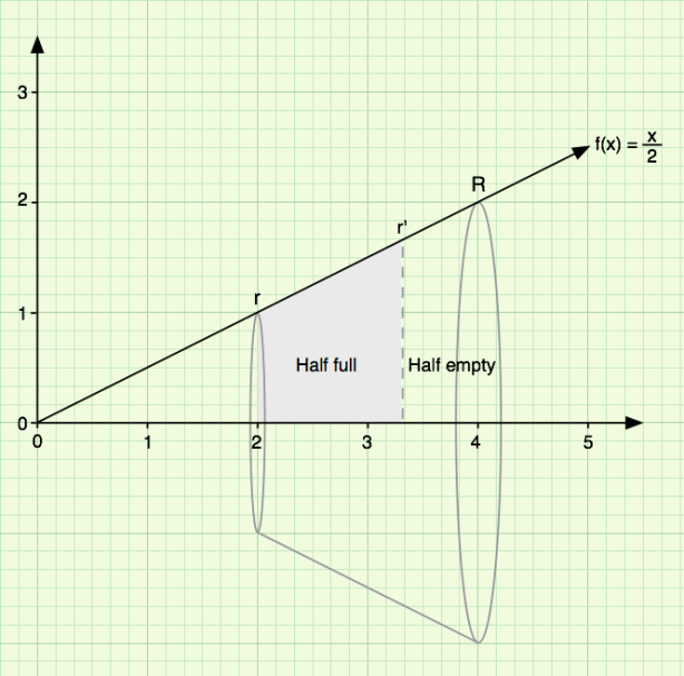
First, let’s design a glass from an easy function:

glass_half_empty_half_full


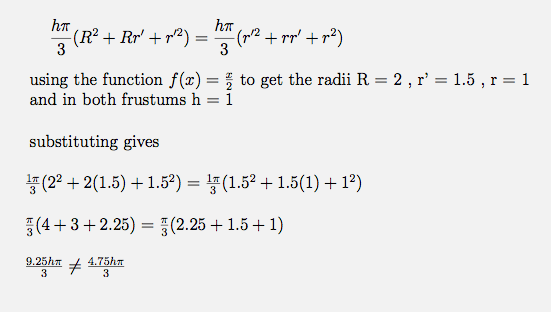
I’m going to divide the glass in two exactly at half its height. The question is, do both halves contain the same amount of water? To answer that use the formula found on the wikipedia page:

two_frustums

So where along the x-axis is half full? There are a couple of ways to approach this question but since we’re already thinking about the above diagram as a solid of revolution and with a little programming a general approach for all glasses can be devised.

The basic idea is to derive the definite integral of the function so that by setting the limits appropriately we can find the total volume and search for the x value that evaluates to half the total volume. The integrations of two functions (the one above and another for a more curved glass) can be seen here. The formulas are coded into the following script:

python_script

When this script is executed the output is:

lower_bound = 2.000000
upper_bound = 4.000000
height      = 2.000000
volume      = 14.660766
half-volume = 7.330383
Tolerance : 0.000001

Iterations: 23
lower_bound = 2.000000
upper_bound = 3.301927
height      = 1.301927
volume      = 7.330384

So the x-axis value which divides the glass into two equal volumes is the lower bound plus the height of 1.301927 or 3.301927. Checking the math using this new value gives:

last_check

Well, ok, they aren’t exactly equal . . . the difference is 3.708323 X 10^-6. Close enough. The glass with the correct amount of fluid in it would look like the following.

really_half_full

Common Core Math

My understanding of the Common Core State Standard Initiative is that it is a set of guidelines as to what students are supposed to learn at various grade levels. How those guidelines are met is left to the individual states that adopt the CCSSI. You can read more here and judge for yourself. I’m not here to argue whether the CCSSI is good or bad, or if it impinges on “States Rights” or if it’s a tool of Satan. I just want to address one REALLY BAD piece of pedagogy.

I recently ran across the following image in a Facebook posting complaining about the Common Core Math requirements.

Common-Core-Math

I can’t find the original, full image so I’m going to interpret the missing text this way:

“Add 26+17 by breaking up the numbers to make a tens group. Use a number that adds to the 6 in 26 to make a 10’s. Since 6+4=10, use 4.”

I’m also assuming that this is the entirety of the problem. The rest is (not so) obvious. In fact it’s mind swivelingly hard to interpret. So for all you parents suffering through addition problems like this here’s my explanation.

For all of us who learned addition between the beginning of time through the “New Math” of the 1960’s the problem can be solved thusly:

Six plus seven is thirteen. Write down the three and carry the one to
the tens place. One plus two plus one is four. Write down the four
giving forty three.

The method in the image is basically asking what number can we add to 26 to force the carry of a one. Well, that would be four. That gets us to thirty but what about the 17? Since we already added four to 26 we have to adjust the 17 down by four before adding it to the 30. That’s where the “17 = 4 + 13” comes from.

Still a little fuzzy? Can you imagine asking a first or second grader, “Use a number that adds to the 6 in 26 to make a 10’s”? I was the little turkey that would always ask, “Why?” That hopefully would lead to a discussion of the carry operation. But this example doesn’t go there. It states, “Think: 17=4+13.” This is a complete non sequitur and doesn’t engage the student in any sort of problem solving activity. It commands “Think” and doesn’t address rational stepwise solution. So, if you’re fuzzy don’t worry.

This is how I would break the problem down (if for some completely twisted reason I was going to teach addition this way . . . which I wouldn’t).

We are going to use a non-traditional method to add the two digit numbers 26 and 17.

  1. First we’re going to find a number that when added to 26 causes a carry into the ten’s place.
  2. Isolate the 6 and solve the following equation:
    6+x=10
    x=10-6
    x=4
  3. Add 4 to 26. Using the “Old Math”, six plus four is ten, write down the zero and carry the one. One plus two is three giving thirty.
  4. Because we adjusted 26 up by 4 (forcing the carry) we must adjust the 17 down by 4. This is where the “17=4+13” comes from. In fact this should be “17-4=13” since that’s the actual computation we need to do . . . but I guess subtraction isn’t covered until next week so we have to “Think” our way around it.
  5. Now we can add the 13 to the 30 and get 43.

So actually all we’re doing is adjusting one number up to the next multiple of 10 and adjusting the second number down by the same factor before adding. Reverse the above problem: 17+26. You can almost do it in your head. (17+3)+(26-3) = 20+23 = 43.

I have several issues with the method.

  1. It only works for two digit numbers. Since it only addresses the carry from the units place this method fails to accurately add three, four, or five digit numbers. It’s not general. Want to make a kid cry? Tell them to use this method to add 998+427.
  2. It works for negative numbers but is potentially very confusing due to the adding of negative numbers. (I forget when I learned about adding negatives – I doubt it was first grade.)
  3. I’m being a stickler here but you just can’t pull the six out of 26 and operate on it. Intuitively you can but formally you have to isolate it with a modulo operation.

Since I spent the time pulling the method out of this horrid bit of pedagogy I might as well formalize it a bit. Here goes.

If x and y are two, two digit integers to be added together the following equation will produce satisfactory answers.

sum = (10 - x mod 10) + x + y - (10 - x mod 10)
where x mod 10 is the remainder after division, e.g. 17 mod 10 = 7.

Ok, need a laugh? Think things are tough now? Here’s a song from the 1960’s by Tom Lehrer. Click here to enjoy.

NCSE/UNC Spectrum Concert

The North Carolina Saxophone Ensemble and the UNC Saxophone Studio will perform on 11Apr2014 in the Kenan Music building rehearsal hall. The program notes for the concert will be projected on a large screen rather than printed, saving paper and allowing people to review the program both before and after the performance. To see the program notes click here.

Here are short descriptions of each piece.

Four5 – The fifth in a series of pieces for four players by John Cage. Cage wrote the “Number Pieces” later in his career. Click here for more information.

Melodies for Saxophone – Thirteen melodies written by Philip Glass for Jean Genet’s play “Prisoner Of Love” adapted by Joanne Akalaitis for the New York Theater Workshop.

The Difficulties – Electronica by Mark Engebretson and poetry by Brian Lampkin. For this performance a jazz baritone saxophone improvisation triggers electronic sounds to compliment the reading of Lampkin’s poem “The Difficulties”.

Far Away – Takatsugu Muramatsu is most noted for his work in film and television but “Far Away” was originally written for the Libera boys choir.

Last Tango in Bayreuth – Peter Schickele originally played this on piano as something of a party trick, eventually completing it as a quartet for four bassoons. It’s a tongue-in cheek tribute to Richard Wagner based on the “Tristan” chord from Tristan ind Isolde and a theme from “Overture to Act III” of Loehengrin.

Shetland Sequence – An arrangement of Shetland jigs by the British saxophonist Jan Steele. The jigs included are “Jack broke da prison door”, “Donald Blue”, “Sleep sound ida morning'”, “Lassies trust in providence”, and “Bonnie Isle o’Whaljay”.

Ecstatic Fanfare – An arrangement of the brass fanfare from the first movement of Steven Bryant’s “Ecstatic Waters” for wind ensemble.

Smiles and Chuckles / Beautiful Ohio Blues – These two pieces date from the early 20th century and were written for the Columbia Saxophone Sextet and The Six Brown Brothers. The arranger, David Lovrien, transcribed the pieces from recordings made on wax cylinders making these truly authentic saxophone pieces.

Capriol Suite – A collection of six dances with a Renaissance flavor written in 1926 by Peter Warlock. Originally written as a piano duet, Warlock re-scored the work for orchestra.

Festive Overture, Opus 96 –  Dmitri Shostakovich wrote this work in three days for the 37th anniversary of the October Revolution in 1954. Stylistically it is based on Glinka‘s Russlan and Ludmilla overture written in 1842.

Trilogy – A transcription of the opening vocal section of the larger work of the same name by Keith Emerson and Greg Lake with the tenor sax taking the vocal solo and the ensemble covering the piano parts.


Complete the Cone – Fact or Myth

I attended the U.S. Navy International Saxophone Symposium at George Mason University earlier this month. Along with all the great recitals and concerts, I attended an excellent  presentation titled “Working With Your Repair Technician” by Shelly Tanabe, owner of  Wind Player Services in NYC. One of the last slides of the presentation addressed the idea that the sax is a conical instrument and that the volume of the mouthpiece completes the cone.

Deep down, I’ve always been suspicious of this idea and seeing it again in the presentation made me decide to investigate it a little deeper. Since it’ll probably take more than one post I’ll add a menu item on the banner titled “Complete the Cone Series” that will link to everything.

Those of you who know me and my background are probably groaning right now. Yes, there will be geometry, trigonometry, and even some 9th grade physical science. Come on, it’ll be fun!!