In our last exciting episode . . .

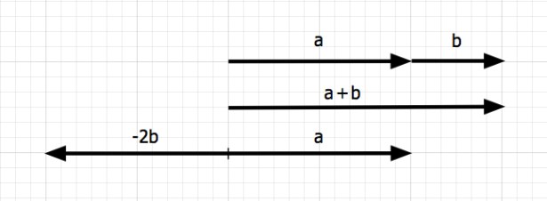
. . . we made an assumption that the slopes of the two vectors – the vector defining the polar plot and its first derivative – would at some point match. That makes sense but isn’t very formal. Refer to the diagram below for the following discussion.

Vectors have direction and magnitude and can be added giving a third vector. The co-linear vectors a and b have magnitudes 12 and 6 units and add together to form a single vector with the same direction but with a magnitude of 18 units. You can also multiply vectors with scalar values to change their directions and magnitudes. In the bottom example I’ve multiplied the b vector by -2 flipping its direction and doubling its magnitude to 12. And of course when you add 12 and -12 you get zero.

NOTE:  In the previous diagram (Fig. 3), for clarity, I drew the tangent vector emanating from the tip of the vector defining the polar – in fact it’s rooted at (0,0) too.

So! We have two vectors both of which are rooted at (0,0). They will be co-linear when the vector defining the polar terminates at the point on the curve that forms a tangent line between (0,0) and the curve. At that point there is a real number that we can multiply one of the vectors by to get them to cancel out to zero – we’ll call than number “u“. Here’s the algebra:

We’ve now derived the same equation two different ways which makes me feel confident that we can use it to determine the best speed to fly. The next thing that needs to happen is to get some real data and use linear regression to determine the values of A, B, C, D, and E.

The details of getting that data will be the subject of the next section.

Next: Perfect Data