The last thing we need to find is the speed to fly. If you remember, back in “The Hairy Part” we used vector calculus to derive an equation for the speed to fly. Just to refresh everyone’s memory, here it is:

We have the values for A, B, C and E from R’s linear model function so we can substitute those in to give us:

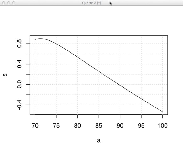
Here I’ve taken the liberty to substitute a for t since we’ve been using a for our airspeeds. Inspecting the factory polar we can see the speed to fly is somewhere around 90 km/hr so let’s plot the above equation for airspeeds from 70 to 100 km/hr. Here’s the R log:

The blow-by-blow for the above is the first line generates airspeeds from 70 through 100, one tenth of a km/hr at a time. The second line defines stf as a function consisting of our equation. This is done to save typing (only have to put the equation in once), and make the rest of the R commands clearer. The third line uses our defined function to generate a “sink” value for every airspeed value. Then we plot it and put a grid on the plot so we can see where zero lies. The ‘type=”l”‘ parameter for the plot says to NOT plot the points but to plot a line segment between each a/s pair. This gives an appearance of a smooth curve.

The plotted line crosses zero just shy of 90 km/hr. Unfortunately we can’t use the maximum value like we did for minimum sink. We could redo the plot from 85 to 95 km/hr and get a better estimate of where the line crosses zero, then expand the scale again say from 88 to 90 km/hr but R gives us a better way.

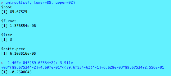
Solve the equation for zero. R has a very handy function for solving one dimensional functions called uniroot. Here’s all there is to it:

The various numbers are where the function is “equal to zero”, the value of the function when it’s evaluated at that value, the number of attempts uniroot took to find the solution and a measure of the precision of the answer (smaller is better). As you can see 89.67529 doesn’t exactly evaluate to zero but 1.376554×10^-6 which is pretty close. If we wanted to get a more precise answer, for some twisted reason, there’s a tolerance parameter we could pass to uniroot to tell it to continue searching until it’s met the tolerance.

The last line – the big ugly expression – is just the solution substituted back into the original model to get the sink rate at the best speed to fly. It’s not very edifying and the factory spec sheet doesn’t say anything about the best speed to fly or the sink rate; you have to divine it from the polar. It does state that the L/D is 33.5 and we can calculate that ourselves from our solution and sink rate.

The first thing we need to do though is get all the numbers in the same units. The easiest thing to do is convert -0.7508645 m/s to km/hr. (No I’m not going to do that here. There are conversion factors on the web and it’s a simple multiply. Or, you can get a conversion app for your smartphone that’ll do it.) The converted sink rate is 2.703112 km/hr. So if you fly at 89.67529 km/hr for an hour you’ll sink 2.703112 km. Sounds like you can get your Lift/Drag ratio from that right? Just divide the sink rate into the speed, all the units cancel and you have the unit-less L/D.

Doing that little bit of arithmetic gives us a L/D of 33.1748 – not bad given the potential measurement errors in generating the data.

Now that we have a process for getting the relevant performance numbers, I’m going to investigate that “too good” fit and do this whole process on another sailplane’s polar to see how the model holds up.