Now that we have a vector based framework to work with we need to come up with an equation that models the polar curve. There are two drag components that work on all aircraft. One is the drag from the cross sectional area (frontal area) of the aircraft moving through the air and the other is the induced drag from the wing producing lift. There’s an equation for each of them:

Don’t throw up your hands yet!! The only things of concern are the velocity terms, everything else is either an environmental variable (e.g., air density) or is particular to the aircraft (e.g., aspect ratio). The one thing we will take away from these equations is that the force of drag is proportional to the square of the velocity and the induced drag is proportional to the inverse square of the velocity.

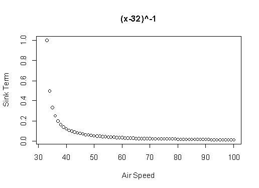
Now with that said I am going to use one aircraft specific number – stall speed. I don’t feel too bad about this because it’s an easy value to find, as opposed to a value like the wing span efficiency value or the sailplane’s drag coefficient. The term built using the stall speed looks like the title on the following graph which assumes a stall speed of 32kts:

As you slow down and approach the stall speed the value of this term gets large very quickly. This makes physical sense – as the stall speed is approached induced drag increases as an inverse proportion and the sink rate quickly increases. This term just defines the bottom limit of our airspeed.

So finally, here’s the equation that we hope models our polar curves:

A through E are coefficients that will later be found via some type of regression analysis. The first three terms are the force of drag, induced drag, our adjustment for the particular aircraft’s stall speed (s) plus a linear term and a regression constant.

Now we have to do a bit of calculus and some unfortunately hairy looking algebra to get the final equations we need to determine our minimum sink and best speed to fly.

Next: The Hairy Part